


Executive Summary
Reason Foundation’s Annual Highway Report has tracked the performance of the 50 state-owned highway systems from 1984 to 2015, using various metrics and methodologies. This edition, the 23rd Annual Highway Report, ranks the performance of state highway systems in 2015, with congestion data from 2016. Each state’s overall rating is determined by rankings in 11 categories, including highway expenditures per mile, Interstate and rural primary road pavement conditions, bridge conditions, urbanized area congestion, fatality rates, and narrow rural arterial lanes. The study is based on spending and performance data state highway agencies submitted to the federal government.
This study also reviews changes in highway performance since 2013, the prior report’s focus.
Although individual state highway sections (roads, bridges, pavements) steadily deteriorate over time due to age, traffic and weather, they are periodically improved by maintenance and reconstruction. As a result, system performance can improve even as individual roads and bridges deteriorate. Table ES1 summarizes recent system trends for key indicators. Despite a decades-long trend of steady, incremental improvement, from 2013 to 2015, the overall condition of the total system, viewed nationally, has worsened. While both rural and urban Interstate pavement conditions have improved, the other eight measures for the U.S. state-owned highway system were worse in 2015 than in 2013. (The congestion metric used in this report is new and cannot be compared to previous measures.)
Table ES1: Tracking the Performance of State-Owned Highways, 2012–2015
| Statistic | 2012 | 2013 | 2015*+ | Percent Change 2013–15 | Percent Change 2012–15 |
|---|---|---|---|---|---|
| Mileage under State Control (Thousands) | 814,284 | 815,024 | 814,154 | -0.11 | -0.02 |
| Total Disbursements per Mile, $ | 162,202 | 160,997 | 178,116 | 10.63 | 9.81 |
| Disbursements per Mile, Capital/Bridges, $ | 86,153 | 84,494 | 91,992 | 8.87 | 6.78 |
| Disbursements per Mile, Maintenance, $ | 26,079 | 25,996 | 28,020 | 7.79 | 7.44 |
| Disbursements per Mile, Administration, $ | 10,579 | 10,051 | 10,864 | 8.09 | 2.7 |
| Consumer Price Index (1984=1.00) | 2.21 | 2.24 | 2.28 | 1.75 | 3.24 |
| Rural Interstate, Percent Poor Condition | 1.78 | 2 | 1.85 | -7.74 | 3.69 |
| Urban Interstate, Percent Poor Condition | 4.97 | 5.37 | 5.02 | -6.52 | 1.04 |
| Rural Other Principal Arterial, Percent Poor Condition | 0.89 | 1.27 | 1.35 | 6.44 | 51.87 |
| Urbanized Area Congestion | NA | **51.40 | ***34.95 | NA | NA |
| Bridges, Percent Deficient | 21.52 | 20.44 | 21.65 | 5.92 | 0.62 |
| Fatality Rate per 100 Million Vehicle-Miles | 1.13 | 1.1 | 1.13 | 3.49 | 0.26 |
| Rural Other Principal Arterial, Percent Narrow Lanes | 8.89 | 8.91 | 9.78 | 9.77 | 10.05 |
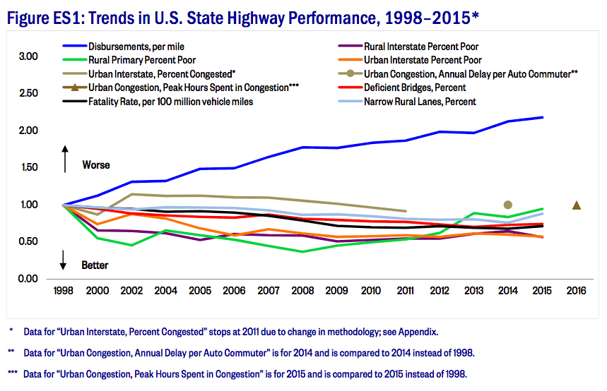
Using similar data metrics and methodologies, Figure ES-1 shows trends in highway performance. Overall, the top rankings continue to be dominated by relatively small rural states. North Dakota led the cost-effectiveness ratings for the first time since 2009, but the state has been in the top 10 for over 20 years. Kansas, South Dakota, Nebraska and South Carolina round out the top five.
Several large states with major cities also fared well: Missouri (9th), North Carolina (14th), Georgia (18th) and Texas (22nd).
At the bottom of the overall rankings are New Jersey, Rhode Island, Alaska, Hawaii and Connecticut.
System performance problems in each measured category seem to be concentrated in a few states:
- Over half (53%) of the rural Interstate mileage in poor condition is in just eight states: Alaska, Colorado, New York, Wisconsin, Indiana, Texas, California and Washington.
- Over half (54%) of the urban Interstate mileage in poor condition is in just eight states: California, New York, Texas, Louisiana, Michigan, New Jersey, Pennsylvania and Ohio.
- Almost half (49%) of the rural primary mileage in poor condition is in just eight states: California, Alaska, Wisconsin, Iowa, Texas, Minnesota, Oklahoma and South Dakota.
- Automobile commuters in nine states (New Jersey, California, New York, Georgia, Illinois, Massachusetts, Texas, Washington and Virginia) spend more than the national average of 35 hours annually stuck in peak-hour traffic congestion.
- Although a majority of states saw bridge conditions improve, overall national bridge conditions are worsening, with seven states (Rhode Island, Hawaii, New York, West Virginia, Massachusetts, Pennsylvania and Connecticut) now reporting more than one-third of their bridges as deficient.
- After decades of improvement, fatality rates are increasing and seven states (South Carolina, Montana, Mississippi, Kentucky, Arkansas, Wyoming and Louisiana) now have fatality rates greater than 1.5 per 100 million vehicle-miles travelled.
- Four states (West Virginia, Virginia, Pennsylvania and Vermont) report that more than one-third of their rural principal arterial systems have lanes considered narrow.
While system performance is down overall this year, nearly half of the states (23 of 50) made progress in 2015 compared to 2013. However, a 10-year average of state overall performance data indicates that a few states are finding it difficult to improve. System performance problems seem to be concentrated in these states. There is also increasing evidence that higher-level road systems (Interstates, other freeways and principal arterials) are in better shape than lower-level road systems, particularly local roads.
Part 1
State Highway Performance Ranks
This report continues its annual ratings of state highway systems on cost versus quality, using a methodology developed in the early 1990s by Dr. David T. Hartgen, emeritus professor at the University of North Carolina at Charlotte. Since states have different budgets, system sizes, traffic and geographic circumstances, their comparative performance depends on both system performance and the resources available. To determine relative performance across the country, state highway system budgets (per mile of responsibility) are compared with system performance, state-by-state. States with high ratings typically have better-than-average system conditions (good for road users) along with relatively low per-mile expenditures (good for taxpayers).
The following table shows the overall highway performance of the state highway systems for 2015. This year’s leading states are North Dakota, Kansas, South Dakota, Nebraska and South Carolina. At the other end of the rankings are Connecticut, Hawaii, Alaska, Rhode Island and New Jersey.
As in prior years, the top-performing states tend to be rural states with limited congestion (Tables 1, 2, 3, 4, and Figure 1). But several states with large urban areas also rank highly: Missouri (9th), North Carolina (14th), Georgia (18th) and Texas (22nd). Although it is tempting to ascribe these ratings solely to geographic circumstances, a more careful review suggests that numerous other factors—terrain, climate, geography, truck volumes, urbanization, system age, budget priorities, unit cost differences, state budget circumstances and management/maintenance philosophies, just to name a few—are all affecting overall performance. The remainder of this report reviews the statistics underlying these overall ratings in more detail.
Overall Performance and Cost-Effectiveness Rankings
23rd Annual Highway Report (PDF)
Click a state name for detailed information about its results.
Overall Highway Performance Ratings in Alphabetical Order
Each State’s Highway Performance Rankings in Each Category
| State | Overall | Total Disbursements per mile | Capital & Bridge Disbursements per mile | Maintenance Disbursements per mile | Administrative Disbursements per mile | Rural Interstate Pavement Condition | Urban Interstate Pavement Condition | Rural Arterial Pavement Condition | Urbanized Area Congestion* | Deficient Bridges | Fatality Rates | Narrow Rural Arterial Lanes |
|---|---|---|---|---|---|---|---|---|---|---|---|---|
| Alabama | 17 | 22 | 23 | 1 | 34 | 21 | 10 | 38 | 13 | 26 | 33 | 38 |
| Alaska | 48 | 20 | 32 | 28 | 21 | 48 | 50 | 28 | 8 | 18 | 35 | 19 |
| Arizona | 16 | 40 | 34 | 20 | 45 | 22 | 15 | 4 | 36 | 1 | 41 | 1 |
| Arkansas | 29 | 8 | 12 | 11 | 7 | 36 | 35 | 44 | 11 | 24 | 46 | 45 |
| California | 42 | 43 | 41 | 47 | 46 | 33 | 45 | 46 | 49 | 28 | 14 | 1 |
| Colorado | 31 | 28 | 31 | 33 | 22 | 47 | 22 | 29 | 35 | 8 | 22 | 30 |
| Connecticut | 46 | 44 | 42 | 31 | 50 | 35 | 48 | 26 | 27 | 44 | 6 | 14 |
| Delaware | 19 | 27 | 13 | 35 | 32 | NA | 1 | 12 | 37 | 13 | 34 | 23 |
| Florida | 35 | 49 | 49 | 44 | 41 | 5 | 2 | 6 | 40 | 11 | 42 | 21 |
| Georgia | 18 | 19 | 17 | 15 | 43 | 29 | 7 | 18 | 47 | 9 | 27 | 29 |
| Hawaii | 47 | 45 | 48 | 41 | 33 | NA | 46 | 50 | 20 | 49 | 12 | 40 |
| Idaho | 7 | 17 | 22 | 25 | 13 | 32 | 12 | 15 | 7 | 17 | 36 | 15 |
| Illinois | 28 | 41 | 46 | 38 | 29 | 1 | 3 | 5 | 46 | 7 | 15 | 33 |
| Indiana | 34 | 31 | 37 | 42 | 19 | 43 | 29 | 43 | 25 | 16 | 20 | 32 |
| Iowa | 15 | 21 | 33 | 21 | 12 | 24 | 39 | 25 | 3 | 34 | 17 | 24 |
| Kansas | 2 | 18 | 21 | 13 | 16 | 10 | 6 | 22 | 15 | 6 | 24 | 12 |
| Kentucky | 13 | 14 | 14 | 14 | 1 | 19 | 8 | 20 | 26 | 40 | 47 | 35 |
| Louisiana | 37 | 23 | 16 | 22 | 5 | 42 | 40 | 49 | 31 | 39 | 44 | 26 |
| Maine | 23 | 11 | 9 | 23 | 4 | 6 | 31 | 24 | 12 | 43 | 21 | 42 |
| Maryland | 40 | 47 | 44 | 46 | 35 | 26 | 26 | 41 | 39 | 32 | 9 | 17 |
| Massachusetts | 44 | 48 | 47 | 45 | 49 | 40 | 41 | 35 | 45 | 46 | 1 | 1 |
| Michigan | 32 | 33 | 35 | 30 | 26 | 41 | 19 | 45 | 33 | 33 | 19 | 36 |
| Minnesota | 25 | 26 | 30 | 34 | 23 | 39 | 30 | 39 | 41 | 2 | 3 | 16 |
| Mississippi | 11 | 12 | 15 | 4 | 14 | 37 | 23 | 31 | 16 | 19 | 48 | 10 |
| Missouri | 9 | 5 | 3 | 12 | 3 | 16 | 9 | 19 | 24 | 30 | 26 | 37 |
| Montana | 6 | 6 | 8 | 8 | 18 | 17 | 28 | 8 | 9 | 14 | 49 | 25 |
| Nebraska | 4 | 10 | 10 | 18 | 2 | 11 | 24 | 23 | 10 | 25 | 28 | 9 |
| Nevada | 20 | 24 | 26 | 16 | 42 | 15 | 33 | 11 | 28 | 27 | 32 | 27 |
| New Hampshire | 30 | 32 | 25 | 43 | 38 | 1 | 43 | 2 | 30 | 38 | 7 | 1 |
| New Jersey | 50 | 50 | 50 | 50 | 48 | 31 | 47 | 47 | 50 | 42 | 4 | 1 |
| New Mexico | 24 | 13 | 7 | 2 | 44 | 18 | 14 | 10 | 14 | 4 | 23 | 46 |
| New York | 45 | 46 | 45 | 49 | 40 | 44 | 34 | 48 | 48 | 48 | 8 | 44 |
| North Carolina | 14 | 3 | 4 | 7 | 9 | 14 | 25 | 7 | 22 | 41 | 29 | 41 |
| North Dakota | 1 | 15 | 29 | 3 | 10 | 4 | 18 | 3 | 4 | 15 | 37 | 13 |
| Ohio | 26 | 34 | 38 | 26 | 36 | 28 | 17 | 27 | 23 | 20 | 18 | 34 |
| Oklahoma | 33 | 29 | 27 | 37 | 39 | 38 | 37 | 42 | 18 | 23 | 38 | 20 |
| Oregon | 21 | 35 | 18 | 27 | 30 | 20 | 20 | 30 | 38 | 29 | 30 | 22 |
| Pennsylvania | 41 | 30 | 28 | 32 | 28 | 27 | 36 | 33 | 34 | 45 | 25 | 48 |
| Rhode Island | 49 | 42 | 43 | 48 | 47 | 34 | 49 | 32 | 29 | 50 | 2 | 31 |
| South Carolina | 5 | 2 | 1 | 10 | 6 | 9 | 21 | 16 | 17 | 21 | 50 | 28 |
| South Dakota | 3 | 4 | 6 | 5 | 17 | 13 | 32 | 14 | 5 | 31 | 43 | 8 |
| Tennessee | 12 | 16 | 20 | 19 | 24 | 7 | 5 | 9 | 32 | 12 | 31 | 39 |
| Texas | 22 | 38 | 39 | 29 | 11 | 23 | 16 | 34 | 44 | 10 | 40 | 18 |
| Utah | 10 | 36 | 19 | 40 | 27 | 8 | 13 | 13 | 19 | 3 | 13 | 1 |
| Vermont | 39 | 25 | 24 | 36 | 37 | 3 | 38 | 1 | 6 | 37 | 5 | 47 |
| Virginia | 27 | 7 | 5 | 24 | 15 | 12 | 4 | 21 | 42 | 36 | 10 | 49 |
| Washington | 43 | 39 | 40 | 39 | 25 | 45 | 27 | 37 | 43 | 35 | 16 | 43 |
| West Virginia | 36 | 1 | 2 | 6 | 8 | 25 | 42 | 17 | 2 | 47 | 39 | 50 |
| Wisconsin | 38 | 37 | 36 | 17 | 31 | 46 | 44 | 40 | 21 | 5 | 11 | 11 |
| Wyoming | 8 | 9 | 11 | 9 | 20 | 30 | 11 | 36 | 1 | 22 | 45 | 1 |
Overall Highway Performance Rating Trends, 2012–2015
| State | 2012 | 2013 | 2015 | 2013–2015 Change in Rank | 2012–2015 Change in Rank |
|---|---|---|---|---|---|
| Alabama | 21 | 20 | 17 | 3 | 4 |
| Alaska | 49 | 50 | 48 | 2 | 1 |
| Arizona | 19 | 24 | 16 | 8 | 3 |
| Arkansas | 35 | 33 | 29 | 4 | 6 |
| California | 45 | 42 | 42 | 0 | 3 |
| Colorado | 33 | 35 | 31 | 4 | 2 |
| Connecticut | 44 | 44 | 46 | -2 | -2 |
| Delaware | 37 | 37 | 19 | 18 | 18 |
| Florida | 31 | 32 | 35 | -3 | -4 |
| Georgia | 13 | 21 | 18 | 3 | -5 |
| Hawaii | 50 | 48 | 47 | 1 | 3 |
| Idaho | 30 | 16 | 7 | 9 | 23 |
| Illinois | 27 | 29 | 28 | 1 | -1 |
| Indiana | 36 | 36 | 34 | 2 | 2 |
| Iowa | 18 | 40 | 15 | 25 | 3 |
| Kansas | 5 | 3 | 2 | 1 | 3 |
| Kentucky | 10 | 14 | 13 | 1 | -3 |
| Louisiana | 40 | 34 | 37 | -3 | 3 |
| Maine | 16 | 5 | 23 | -18 | -7 |
| Maryland | 39 | 38 | 40 | -2 | -1 |
| Massachusetts | 46 | 46 | 44 | 2 | 2 |
| Michigan | 32 | 31 | 32 | -1 | 0 |
| Minnesota | 28 | 27 | 25 | 2 | 3 |
| Mississippi | 8 | 10 | 11 | -1 | -3 |
| Missouri | 12 | 12 | 9 | 3 | 3 |
| Montana | 9 | 6 | 6 | 0 | 3 |
| Nebraska | 2 | 4 | 4 | 0 | -2 |
| Nevada | 24 | 22 | 20 | 2 | 4 |
| New Hampshire | 23 | 26 | 30 | -4 | -7 |
| New Jersey | 48 | 49 | 50 | -1 | -2 |
| New Mexico | 7 | 11 | 24 | -13 | -17 |
| New York | 43 | 45 | 45 | 0 | -2 |
| North Carolina | 20 | 15 | 14 | 1 | 6 |
| North Dakota | 6 | 7 | 1 | 6 | 5 |
| Ohio | 14 | 9 | 26 | -17 | -12 |
| Oklahoma | 22 | 17 | 33 | -16 | -11 |
| Oregon | 26 | 23 | 21 | 2 | 5 |
| Pennsylvania | 41 | 39 | 41 | -2 | 0 |
| Rhode Island | 47 | 47 | 49 | -2 | -2 |
| South Carolina | 4 | 1 | 5 | -4 | -1 |
| South Dakota | 3 | 2 | 3 | -1 | 0 |
| Tennessee | 17 | 18 | 12 | 6 | 5 |
| Texas | 11 | 19 | 22 | -3 | -11 |
| Utah | 29 | 13 | 10 | 3 | 19 |
| Vermont | 38 | 41 | 39 | 2 | -1 |
| Virginia | 25 | 30 | 27 | 3 | -2 |
| Washington | 42 | 43 | 43 | 0 | -1 |
| West Virginia | 34 | 25 | 36 | -11 | -2 |
| Wisconsin | 15 | 28 | 38 | -10 | -23 |
| Wyoming | 1 | 8 | 8 | 0 | -7 |
Figure 1: Overall Highway Performance Rank, 2015
[show-map id=’10’]The overall ranking in 2015 for most states was not dramatically different than the previous edition of this report, despite a new metric of urban area congestion. However, two states saw their overall rankings improve by double digits and six states had overall rankings that worsened by 10 or more spots:
- Iowa improved 25 positions, from 40th to 15th in the overall rankings, as the state’s per mile spending increased somewhat but mileage in poor condition (on urban and rural Interstates and rural arterials) improved considerably.
- Delaware improved 18 spots, from 37th to 19th overall, as per mile spending decreased while mileage in poor condition (on urban Interstates and rural arterials) still improved considerably.
- Wisconsin fell 10 spots, from 28th to 38th, as per mile spending increased even as mileage in poor condition (on urban and rural Interstates) worsened.
- West Virginia fell 11 spots, from 25th to 36th, as the condition of its bridges worsened, as did the condition of its rural Interstates and arterials.
- New Mexico fell 13 spots, from 11th to 24th, as urban area congestion worsened and narrow rural arterial lane mileage increased.
- Oklahoma fell 16 spots, from 17th to 33rd, as per mile spending increased even as mileage in poor condition (on urban and rural Interstates and rural arterials) worsened considerably.
- Ohio fell 17 spots, from 9th to 26th, as per mile spending increased but the state’s road conditions worsened. Additionally, Ohio’s percentage of bridges in deficient condition jumped considerably as this year’s totals included functionally obsolete bridges, whereas in the last assessment, this information was not provided.
- Maine fell 18 spots, from 5th to 23rd, as per mile spending increased even as the state’s road conditions (particularly urban Interstates) worsened.
Part 2
Background Data
State highway system sizes range from approximately 1,000 miles to more than 80,000 miles. States with larger geographic areas and larger populations tend to have larger systems. Some states, such as North Carolina, maintain all of their roads on the state level, except for subdivision and other local roads. Other states, such as Florida, have robust county road systems. State-controlled highway mileage and state highway agency miles are not included directly in the rankings. They are included in this report as background information and are used to weight the financial data.
State-Controlled Miles
State-controlled mileage includes the state highway systems, state-agency toll roads, some ferry services, and smaller systems serving universities and state-owned properties. It includes the Interstate System, the National Highway System, and most federal aid system roads. Nationwide in 2015, about 814,154 miles were under state control (Table 5, State-Controlled Highway Mileage), about 870 miles fewer than in 2013 (815,024), the last time this assessment was completed. Small annual changes in state-controlled miles are to be expected, as state systems are expanded to meet increasing needs, but sometimes jurisdictions assume responsibility for mileage previously under state control. The smallest state-owned road systems continue to be Hawaii (1,012 miles) and Rhode Island (1,158 miles); the largest are Texas (80,794 miles) and North Carolina (80,597 miles).
State-Controlled Highway Mileage
| 2015 Rank | State | Mileage |
|---|---|---|
| 1 | Texas | 80,794 |
| 2 | North Carolina | 80,597 |
| 3 | Virginia | 58,687 |
| 4 | South Carolina | 41,554 |
| 5 | Pennsylvania | 41,105 |
| 6 | West Virginia | 34,685 |
| 7 | Missouri | 33,983 |
| 8 | Kentucky | 28,197 |
| 9 | Ohio | 20,363 |
| 10 | Georgia | 18,070 |
| 11 | Illinois | 16,777 |
| 12 | Louisiana | 16,723 |
| 13 | New York | 16,527 |
| 14 | Arkansas | 16,423 |
| 15 | California | 16,192 |
| 16 | Washington | 15,431 |
| 17 | Tennessee | 14,276 |
| 18 | Minnesota | 13,525 |
| 19 | Oklahoma | 13,358 |
| 20 | Florida | 12,203 |
| 21 | New Mexico | 12,130 |
| 22 | Indiana | 11,770 |
| 23 | Wisconsin | 11,746 |
| 24 | Mississippi | 11,539 |
| 25 | Montana** | 11,352 |
| 26 | Alabama | 11,089 |
| 27 | Kansas | 10,530 |
| 28 | Nebraska | 10,062 |
| 29 | Colorado | 9,914 |
| 30 | Michigan | 9,752 |
| 31 | Iowa | 9,499 |
| 32 | South Dakota | 9,439 |
| 33 | Oregon | 9,134 |
| 34 | Maine | 8,652 |
| 35 | Alaska | 7,959 |
| 36 | Wyoming | 7,949 |
| 37 | North Dakota | 7,426 |
| 38 | Arizona** | 7,214 |
| 39 | Utah | 6,393 |
| 40 | Delaware | 5,481 |
| 41 | Nevada | 5,450 |
| 42 | Maryland | 5,443 |
| 43 | Idaho* | 4,992 |
| 44 | Connecticut | 4,054 |
| 45 | New Hampshire | 4,008 |
| 46 | Massachusetts | 3,556 |
| 47 | New Jersey | 3,352 |
| 48 | Vermont | 2,629 |
| 49 | Rhode Island | 1,158 |
| 50 | Hawaii | 1,012 |
| U.S. Total | 814,154 | |
| Average | 16,283 |
State Highway Agency (SHA) Miles
State highway agency roads are generally the Interstates and other major US-numbered and state-numbered roads. A few states also manage major portions of the rural road system. In 2015, about 779,457 miles were the responsibility of the 50 State Highway Agencies (Table 6, State Highway Agency Mileage), about 222 more miles than in 2013 (779,235), the last time this assessment was completed. The average number of lanes per mile is 2.40 lanes, but a few states (New Jersey, Florida, California and Massachusetts) manage significantly wider roads, averaging more than 3.0 lanes per mile.
State Highway Agency Mileage, by average number of lanes/mile
| Rank | State | SHA Miles | SHA Lane-Miles | Ratio |
|---|---|---|---|---|
| 1 | West Virginia | 34,403 | 70,987 | 2.06 |
| 2 | Maine | 8,358 | 17,548 | 2.1 |
| 3 | Alaska | 5,611 | 11,906 | 2.12 |
| 4 | New Hampshire | 3,902 | 8,405 | 2.15 |
| 5 | North Carolina | 79,559 | 171,687 | 2.16 |
| 6 | Virginia | 58,648 | 127,258 | 2.17 |
| 7 | South Carolina | 41,359 | 90,465 | 2.19 |
| 8 | Delaware | 5,402 | 11,859 | 2.2 |
| 9 | Pennsylvania | 39,756 | 88,297 | 2.22 |
| 10 | Kentucky | 27,636 | 61,987 | 2.24 |
| 11 | Missouri | 33,873 | 76,289 | 2.25 |
| 12 | Nebraska | 9,941 | 22,508 | 2.26 |
| 13 | Montana | 11,014 | 25,125 | 2.28 |
| 14 | Vermont | 2,629 | 6,003 | 2.28 |
| 15 | Arkansas | 16,423 | 37,640 | 2.29 |
| 16 | South Dakota | 7,766 | 17,921 | 2.31 |
| 17 | North Dakota | 7,406 | 17,217 | 2.32 |
| 18 | Kansas | 10,292 | 23,996 | 2.33 |
| 19 | Wyoming | 6,718 | 15,726 | 2.34 |
| 20 | Louisiana | 16,689 | 39,332 | 2.36 |
| 21 | Oregon | 7,661 | 18,594 | 2.43 |
| 22 | Texas | 80,423 | 195,756 | 2.43 |
| 23 | New Mexico | 11,976 | 29,504 | 2.46 |
| 24 | Idaho | 4,992 | 12,341 | 2.47 |
| 25 | Oklahoma | 12,257 | 30,356 | 2.48 |
| 26 | Minnesota | 11,811 | 29,260 | 2.48 |
| 27 | Wisconsin | 11,746 | 29,669 | 2.53 |
| 28 | Nevada | 5,380 | 13,598 | 2.53 |
| 29 | Colorado | 9,061 | 22,928 | 2.53 |
| 30 | New York | 15,049 | 38,320 | 2.55 |
| 31 | Iowa | 8,880 | 22,739 | 2.56 |
| 32 | Ohio | 19,228 | 49,416 | 2.57 |
| 33 | Mississippi | 10,901 | 28,075 | 2.58 |
| 34 | Indiana | 11,169 | 28,769 | 2.58 |
| 35 | Rhode Island | 1,091 | 2,848 | 2.61 |
| 36 | Washington | 7,058 | 18,478 | 2.62 |
| 37 | Hawaii | 942 | 2,487 | 2.64 |
| 38 | Connecticut | 3,720 | 9,832 | 2.64 |
| 39 | Illinois | 15,967 | 42,235 | 2.65 |
| 40 | Tennessee | 13,878 | 37,220 | 2.68 |
| 41 | Alabama | 10,920 | 29,568 | 2.71 |
| 42 | Georgia | 17,949 | 49,074 | 2.73 |
| 43 | Utah | 5,871 | 16,127 | 2.75 |
| 44 | Michigan | 9,668 | 27,444 | 2.84 |
| 45 | Maryland | 5,154 | 14,763 | 2.86 |
| 46 | Arizona | 6,822 | 19,612 | 2.87 |
| 47 | Massachusetts | 2,945 | 9,302 | 3.16 |
| 48 | California | 15,093 | 51,686 | 3.42 |
| 49 | Florida | 12,116 | 43,759 | 3.61 |
| 50 | New Jersey | 2,340 | 8,555 | 3.66 |
| U.S. Total | 779,457 | 1,874,470 | 2.4 | |
| Weighted Average | 15,589 | 37,489 |
Part 3
Performance Indicators
The Annual Highway Report ranks each state in 11 categories. Four of the categories measure spending: Capital and Bridge Disbursements, Maintenance Disbursements, Administrative Disbursements and Total Disbursements. Seven of the categories measure highway system performance: Rural Interstate Pavement Condition, Urban Interstate Pavement Condition, Rural Other Principal Arterial Pavement Condition, Urban Area Congestion, Deficient Bridges, Fatality Rates and Narrow Rural Other Principal Arterial Lanes.
The four spending categories are considered together, weighted equally and then averaged to get one overall spending score. The seven performance categories are also considered together, weighted equally and then averaged to get one overall performance score. Then the spending and performance composite scores are added together, weighted by the number of metrics, and averaged to create one total score for each state. Therefore each measure, whether spending efficiency or system performance, is weighted equally.
Detailed data and trends in rankings for each of the states are shown in the attached tables. Selected system condition measures are also shown in the attached maps.
Capital and Bridge Disbursements
Capital and bridge disbursements are the costs to build new, and widen existing, highways and bridges. Capital and bridge disbursements for state-owned roads make up 51.6% of total disbursements, totaling $74.90 billion in 2015, about 8.8% more than was spent in 2013 ($68.86 billion), the last time this assessment was completed.
On a per-mile basis, capital and bridge disbursements increased about 8.9%, from $84,494 per mile in 2013 to $91,992 per mile in 2015 (Table 7, Capital and Bridge Disbursements per State-Controlled Mile, 2015). This increase continues a generally upward trend in spending over the last decade. Since 2006, these per-mile disbursements have increased over 37%, while the Consumer Price Index (CPI) has increased about 18%.
In 2015, South Carolina, West Virginia, Missouri and North Carolina reported the lowest per-mile capital and bridge expenditures. New Jersey, Florida, Hawaii and Massachusetts reported the highest per-mile expenditures. The states with the largest percentage shifts from 2013 to 2015 were Hawaii and New York (which increased per-mile expenditures by more than 49%) and Washington and South Dakota (which decreased per-mile expenditures by more than 34%). Some of the disbursements per state-controlled mile can vary widely from year to year—reflecting funding actions and project schedules.
Capital and Bridge Disbursements Per State-Controlled Mile
| Rank | Name | Dollars |
|---|---|---|
| 1 | South Carolina | $15,675 |
| 2 | West Virginia | $18,857 |
| 3 | Missouri | $25,598 |
| 4 | North Carolina | $29,441 |
| 5 | Virginia | $31,242 |
| 6 | South Dakota | $33,288 |
| 7 | New Mexico | $36,754 |
| 8 | Montana | $39,979 |
| 9 | Maine | $46,947 |
| 10 | Nebraska | $48,712 |
| 11 | Wyoming | $51,248 |
| 12 | Arkansas | $51,958 |
| 13 | Delaware | $56,307 |
| 14 | Kentucky | $61,500 |
| 15 | Mississippi | $62,128 |
| 16 | Louisiana | $63,170 |
| 17 | Georgia | $64,648 |
| 18 | Oregon | $68,801 |
| 19 | Utah | $71,924 |
| 20 | Tennessee | $72,418 |
| 21 | Kansas | $72,948 |
| 22 | Idaho | $73,442 |
| 23 | Alabama | $74,649 |
| 24 | Vermont | $77,441 |
| 25 | New Hampshire | $77,762 |
| 26 | Nevada | $81,303 |
| 27 | Oklahoma | $82,996 |
| 28 | Pennsylvania | $86,394 |
| 29 | North Dakota | $87,710 |
| 30 | Minnesota | $90,640 |
| 31 | Colorado | $93,264 |
| 32 | Alaska | $99,573 |
| 33 | Iowa | $106,120 |
| 34 | Arizona | $109,047 |
| 35 | Michigan | $111,002 |
| 36 | Wisconsin | $117,191 |
| 37 | Indiana | $120,395 |
| 38 | Ohio | $134,201 |
| 39 | Texas | $146,634 |
| 40 | Washington | $153,170 |
| 41 | California | $189,345 |
| 42 | Connecticut | $206,515 |
| 43 | Rhode Island** | $213,079 |
| 44 | Maryland | $251,799 |
| 45 | New York | $259,948 |
| 46 | Illinois | $263,315 |
| 47 | Massachusetts* | $299,246 |
| 48 | Hawaii | $316,637 |
| 49 | Florida | $454,676 |
| 50 | New Jersey | $919,040 |
| Weighted Average | $91,992 |
Maintenance Disbursements
Maintenance disbursements are the costs to perform routine upkeep, such as filling in potholes and repaving roads. Maintenance disbursements comprise about 15.7% of total disbursements, totaling $22.81 billion in 2015, about 7.6% more than in 2013 ($21.19 billion), the last time this assessment was completed.
On a per-mile basis, maintenance disbursements averaged about $28,020 per state, up 7.8% from $25,996 in 2013 (Table 8, Maintenance Disbursements per State-Controlled Mile, 2015). This increase continues a generally upward trend over the last decade. Since 2006 per-mile maintenance disbursements have increased about 34%, relative to a 46% increase in total disbursements and an 18% increase in the Consumer Price Index (CPI). The lowest per-mile maintenance disbursement was $2,692 in Alabama, the highest was $208,736 per mile in New Jersey.
Maintenance Disbursements Per State-Controlled Mile"
| Rank | Name | Dollars |
|---|---|---|
| 1 | Alabama | $2,692 |
| 2 | New Mexico | $3,856 |
| 3 | North Dakota | $4,088 |
| 4 | Mississippi | $6,639 |
| 5 | South Dakota | $8,299 |
| 6 | West Virginia | $9,055 |
| 7 | North Carolina | $10,964 |
| 8 | Montana | $11,571 |
| 9 | Wyoming | $11,807 |
| 10 | South Carolina | $12,397 |
| 11 | Arkansas | $12,895 |
| 12 | Missouri | $13,942 |
| 13 | Kansas | $15,515 |
| 14 | Kentucky | $17,168 |
| 15 | Georgia | $19,271 |
| 16 | Nevada | $20,262 |
| 17 | Wisconsin | $20,412 |
| 18 | Nebraska | $21,160 |
| 19 | Tennessee | $22,120 |
| 20 | Arizona | $22,618 |
| 21 | Iowa | $23,759 |
| 22 | Louisiana | $24,285 |
| 23 | Maine | $24,619 |
| 24 | Virginia | $24,926 |
| 25 | Idaho | $25,265 |
| 26 | Ohio | $25,379 |
| 27 | Oregon | $26,919 |
| 28 | Alaska | $28,545 |
| 29 | Texas | $28,632 |
| 30 | Michigan | $32,152 |
| 31 | Connecticut | $35,384 |
| 32 | Pennsylvania | $35,519 |
| 33 | Colorado | $36,695 |
| 34 | Minnesota | $40,783 |
| 35 | Delaware | $42,949 |
| 36 | Vermont | $45,410 |
| 37 | Oklahoma | $47,769 |
| 38 | Illinois | $48,651 |
| 39 | Washington | $50,199 |
| 40 | Utah | $57,761 |
| 41 | Hawaii | $57,833 |
| 42 | Indiana | $58,183 |
| 43 | New Hampshire | $59,215 |
| 44 | Florida | $80,165 |
| 45 | Massachusetts* | $80,573 |
| 46 | Maryland | $81,912 |
| 47 | California | $84,005 |
| 48 | Rhode Island** | $84,603 |
| 49 | New York | $91,861 |
| 50 | New Jersey | $208,736 |
| Weighted Average | $28,020 |
Administrative Disbursements
Administrative disbursements typically include general and main-office expenditures in support of state-administered highways. They do not include project-related costs but occasionally include “parked” funds, which are funds from bond sales or asset sales awaiting later expenditure. They can therefore vary quite widely from year to year.
Administrative disbursements for state-owned roads totaled $8.8 billion in 2015, about 7.3% more than in 2013 ($8.2 billion), the last time this assessment was completed. This is about 6.1% of the total disbursements. Over the last decade, per-mile administrative disbursements have increased about 26%, less than the 46% increase in total disbursements, but more than the 18% increase in the Consumer Price Index (CPI). On a per-mile basis, 2015 administrative disbursements averaged $10,864 per state, ranging from a low of $1,043 in Kentucky to a high of $99,417 in Connecticut (Table 9, Administrative Disbursements per State-Controlled Mile, 2015).
Administrative Disbursements Per State-Controlled Mile
| Rank | Name | Dollars |
|---|---|---|
| 1 | Kentucky | $1,043 |
| 2 | Nebraska | $2,068 |
| 3 | Missouri | $2,180 |
| 4 | Maine | $2,457 |
| 5 | Louisiana | $2,571 |
| 6 | South Carolina | $2,704 |
| 7 | Arkansas | $3,424 |
| 8 | West Virginia | $3,571 |
| 9 | North Carolina | $3,593 |
| 10 | North Dakota | $3,603 |
| 11 | Texas | $4,082 |
| 12 | Iowa | $5,536 |
| 13 | Idaho | $6,060 |
| 14 | Mississippi | $6,180 |
| 15 | Virginia | $6,195 |
| 16 | Kansas | $6,528 |
| 17 | South Dakota | $6,674 |
| 18 | Montana | $7,019 |
| 19 | Indiana | $7,788 |
| 20 | Wyoming | $10,955 |
| 21 | Alaska | $11,116 |
| 22 | Colorado | $11,190 |
| 23 | Minnesota | $11,342 |
| 24 | Tennessee | $11,791 |
| 25 | Washington | $11,889 |
| 26 | Michigan | $12,374 |
| 27 | Utah | $14,412 |
| 28 | Pennsylvania | $14,769 |
| 29 | Illinois | $15,600 |
| 30 | Oregon | $15,743 |
| 31 | Wisconsin | $16,958 |
| 32 | Delaware | $17,525 |
| 33 | Hawaii | $18,545 |
| 34 | Alabama | $18,977 |
| 35 | Maryland | $19,773 |
| 36 | Ohio | $20,019 |
| 37 | Vermont | $21,467 |
| 38 | New Hampshire | $21,594 |
| 39 | Oklahoma | $21,972 |
| 40 | New York | $23,129 |
| 41 | Florida | $24,371 |
| 42 | Nevada | $24,875 |
| 43 | Georgia | $26,672 |
| 44 | New Mexico | $28,368 |
| 45 | Arizona | $31,576 |
| 46 | California | $36,979 |
| 47 | Rhode Island** | $39,034 |
| 48 | New Jersey | $63,757 |
| 49 | Massachusetts* | $77,086 |
| 50 | Connecticut | $99,417 |
| Weighted Average | $10,864 |
Total Disbursements
Since capital and bridge, maintenance and administrative disbursements make up the majority of expenditures (73.5% in 2015), this report measures them individually and collectively. Total disbursements include those three funding categories, plus three others: Highway Law Enforcement and Safety, Interest, and Bond Retirement. In total, the states disbursed about $145.0 billion for state-owned roads in 2015, a 10.5% increase from $131.2 billion in 2013, the last time this assessment was completed. Over the last decade, highway spending has steadily increased. Since 2006, per-mile total disbursements have increased about 46%, while the Consumer Price Index (CPI) has increased 18%. On a per-mile basis, 2015 disbursements averaged $178,116 (Table 10, Total Disbursements per State-Controlled Mile, 2015). The lowest disbursement per mile was in West Virginia ($35,047) and the highest was in New Jersey ($2,069,020).
Total Disbursements Per State-Controlled Mile
| Rank | Name | Dollars |
|---|---|---|
| 1 | West Virginia | $35,047 |
| 2 | South Carolina | $37,084 |
| 3 | North Carolina | $51,808 |
| 4 | South Dakota | $52,125 |
| 5 | Missouri | $57,481 |
| 6 | Montana | $65,171 |
| 7 | Virginia | $71,829 |
| 8 | Arkansas | $78,179 |
| 9 | Wyoming | $79,348 |
| 10 | Nebraska | $79,397 |
| 11 | Maine | $83,926 |
| 12 | Mississippi | $84,818 |
| 13 | New Mexico | $90,839 |
| 14 | Kentucky | $92,681 |
| 15 | North Dakota | $100,608 |
| 16 | Tennessee | $108,828 |
| 17 | Idaho | $125,328 |
| 18 | Kansas | $145,050 |
| 19 | Georgia | $146,909 |
| 20 | Alaska | $147,699 |
| 21 | Iowa | $149,289 |
| 22 | Alabama | $153,508 |
| 23 | Louisiana | $158,137 |
| 24 | Nevada | $158,542 |
| 25 | Vermont | $171,051 |
| 26 | Minnesota | $174,997 |
| 27 | Delaware | $178,479 |
| 28 | Colorado | $183,224 |
| 29 | Oklahoma | $188,912 |
| 30 | Pennsylvania | $195,633 |
| 31 | Indiana | $196,848 |
| 32 | New Hampshire | $197,468 |
| 33 | Michigan | $207,162 |
| 34 | Ohio | $213,040 |
| 35 | Oregon | $231,096 |
| 36 | Utah | $243,551 |
| 37 | Wisconsin | $250,740 |
| 38 | Texas | $252,744 |
| 39 | Washington | $322,600 |
| 40 | Arizona | $354,473 |
| 41 | Illinois | $376,608 |
| 42 | Rhode Island** | $418,665 |
| 43 | California | $471,052 |
| 44 | Connecticut | $497,659 |
| 45 | Hawaii | $519,237 |
| 46 | New York | $532,538 |
| 47 | Maryland | $578,995 |
| 48 | Massachusetts* | $695,443 |
| 49 | Florida | $744,796 |
| 50 | New Jersey | $2,069,020 |
| Weighted Average | $178,116 |
Rural Interstate Condition
Rural Interstates are typically four- to six-lane roadways connecting urban areas. One measurement of roadway condition is pavement condition. In most states road pavement condition is measured using special machines that determine the roughness of road surfaces. A few states continue to use visual ratings, which are then converted to roughness. In 2015, about 1.85% of U.S. rural Interstates—529 miles out of 28,657—were reported to be in poor condition. (Table 11, Percent Rural Interstate Mileage in Poor Condition, 2015, Figure 2). This is a slight improvement from 2013, the last time this assessment was completed, when 588 miles out of 29,385 (about 2.00%) of rural Interstate pavement was rated poor.
The amount of poor-condition rural Interstate mileage varies widely by state. In 2015, two states reported no poor mileage, and 19 more reported less than 1% poor mileage. On the other hand, four states (Alaska, Colorado, Wisconsin and Washington) reported more than 5% poor mileage. The four states together have about 9% of U.S. rural Interstates (2,592 miles of 28,657), but have over 33% of the poor-condition mileage. Additionally, three states reported a shift of two percentage points or more in the percentage of poor-condition rural Interstate mileage from 2013 to 2015; the amount of poor-mileage increased in Oklahoma, and decreased in California and Washington.
Delaware and Hawaii are the only states with no rural mileage in their Interstate systems.
Percent Rural Interstate Mileage in Poor Condition
| Rank | Name | Percent |
|---|---|---|
| 1 | Illinois | 0 |
| 1 | New Hampshire | 0 |
| 3 | Vermont | 0.12 |
| 4 | North Dakota | 0.12 |
| 5 | Florida | 0.17 |
| 6 | Maine | 0.23 |
| 7 | Tennessee | 0.25 |
| 8 | Utah | 0.29 |
| 9 | South Carolina | 0.39 |
| 10 | Kansas | 0.48 |
| 11 | Nebraska | 0.57 |
| 12 | Virginia | 0.59 |
| 13 | South Dakota | 0.62 |
| 14 | North Carolina | 0.67 |
| 15 | Nevada | 0.7 |
| 16 | Missouri | 0.73 |
| 17 | Montana | 0.79 |
| 18 | New Mexico | 0.81 |
| 19 | Kentucky | 0.82 |
| 20 | Oregon | 0.97 |
| 21 | Alabama | 0.99 |
| 22 | Arizona | 1.14 |
| 23 | Texas | 1.22 |
| 24 | Iowa | 1.24 |
| 25 | West Virginia | 1.39 |
| 26 | Maryland | 1.5 |
| 27 | Pennsylvania | 1.52 |
| 28 | Ohio | 1.52 |
| 29 | Georgia | 1.55 |
| 30 | Wyoming | 1.6 |
| 31 | New Jersey | 1.8 |
| 32 | Idaho | 1.86 |
| 33 | California | 1.87 |
| 34 | Rhode Island | 1.9 |
| 35 | Connecticut | 1.98 |
| 36 | Arkansas | 2.49 |
| 37 | Mississippi | 2.56 |
| 38 | Oklahoma | 2.84 |
| 39 | Minnesota | 3.04 |
| 40 | Massachusetts | 3.27 |
| 41 | Michigan | 3.49 |
| 42 | Louisiana | 3.62 |
| 43 | Indiana | 3.78 |
| 44 | New York | 4.06 |
| 45 | Washington | 5.21 |
| 46 | Wisconsin | 5.44 |
| 47 | Colorado | 5.95 |
| 48 | Alaska | 8.86 |
| 49 | Hawaii * | NA |
| 50 | Delaware * | NA |
| Weighted Average | 1.85 |
Figure 2: Percent of Rural Interstates in Poor Condition, 2015
[show-map id=’11’]Urban Interstate Condition
The urban Interstates consist of major multi-lane Interstates in and near urbanized areas. The pavement condition of the urban Interstate system improved from 2013 to 2015, going from 5.37% in poor condition to 5.02% poor (Table 12, Percent Urban Interstate Mileage in Poor Condition, 2015, Figure 3). In 2015, 940 of the 18,730 miles of urban Interstates were rated as poor, as compared to 945 poor-condition miles out of 17,618 miles in 2013, the last time this assessment was completed.
Between 2013 and 2015, the percentage of poor urban Interstate mileage decreased in 25 states, increased in 21 states and remained about the same in the four remaining states. More than half of the shifts were one percentage point or less. Delaware and Iowa led the states in reducing poor-condition mileage (by 8.4 and 7.7 percentage points, respectively) and Rhode Island, Pennsylvania and Kansas saw increases in poor-condition urban Interstate mileage of three percentage points or more.
The condition of urban Interstate miles also varies widely by state. In 2015, every state reported at least a small percentage of its urban Interstate mileage in poor condition. In the previous 10 years, there often have been states reporting no mileage in poor condition (two in 2012, four in 2011 and nine in 2009). Five states had less than 1% poor mileage (led by Vermont with 0.17) while the bottom five states (California, New Jersey, New York, Louisiana and Hawaii) reported more than 8% poor mileage. These five states, collectively, only have about 16% of the urban Interstate mileage in the U.S. (3,004 of 18,730 miles) but have over 34% of the poor mileage (318 of 940 miles).
Percent Urban Interstate Mileage in Poor Condition
| Rank | Name | Percent |
|---|---|---|
| 1 | Vermont | 0.17 |
| 2 | New Hampshire | 0.48 |
| 3 | North Dakota | 0.62 |
| 4 | Arizona | 0.63 |
| 5 | Illinois | 0.88 |
| 6 | Florida | 1.05 |
| 7 | North Carolina | 1.66 |
| 8 | Montana | 1.71 |
| 9 | Tennessee | 1.76 |
| 10 | New Mexico | 1.83 |
| 11 | Nevada | 1.91 |
| 12 | Delaware | 1.91 |
| 13 | Utah | 2.11 |
| 14 | South Dakota | 2.13 |
| 15 | Idaho | 2.32 |
| 16 | South Carolina | 2.41 |
| 17 | West Virginia | 2.65 |
| 18 | Georgia | 2.77 |
| 19 | Missouri | 2.83 |
| 20 | Kentucky | 2.93 |
| 21 | Virginia | 3.2 |
| 22 | Kansas | 3.26 |
| 23 | Nebraska | 3.39 |
| 24 | Maine | 3.42 |
| 25 | Iowa | 3.43 |
| 26 | Connecticut | 3.56 |
| 27 | Ohio | 3.65 |
| 28 | Alaska | 3.83 |
| 29 | Colorado | 3.91 |
| 30 | Oregon | 4.16 |
| 31 | Mississippi | 4.2 |
| 32 | Rhode Island | 4.81 |
| 33 | Pennsylvania | 5.05 |
| 34 | Texas | 5.15 |
| 35 | Massachusetts | 5.18 |
| 36 | Wyoming | 5.37 |
| 37 | Washington | 6.15 |
| 38 | Alabama | 6.3 |
| 39 | Minnesota | 6.54 |
| 40 | Wisconsin | 6.7 |
| 41 | Maryland | 7.44 |
| 42 | Oklahoma | 7.55 |
| 43 | Indiana | 7.6 |
| 44 | Arkansas | 7.96 |
| 45 | Michigan | 8 |
| 46 | California | 8.72 |
| 47 | New Jersey | 9.79 |
| 48 | New York | 11.21 |
| 49 | Louisiana | 13.66 |
| 50 | Hawaii | 25.13 |
| Weighted Average | 5.02 |
Figure 3: Percent of Urban Interstates in Poor Condition, 2015
[show-map id=’4′]Rural Other Principal Arterial Pavement Condition
The condition of major rural highways worsened slightly from 2013 to 2015, by about 0.08 percentage points. Overall, about 1.35% of the rural other principal arterial (ROPA) system—1,192 miles out of 88,155—was reported to be in poor condition (Table 13, Percent Rural Other Principal Arterial Mileage in Poor Condition, 2015, Figure 4). This compares with about 1.27% (1,126 of 88,550 miles) in 2013, the last time this assessment was completed. This is the highest amount of poor condition mileage since before 2000. (It should be noted that as cities grow, the urbanized area around them grows as well. As this occurs, roads near cities are often reclassified from rural to urban. If these roads were in good condition already, their reclassification has the effect of increasing the percentage of rural roads in poor condition.)
Between 2013 and 2015 most states saw minor changes in ROPA pavement condition. Thirty-five states saw decreases/increases of poor condition mileage of one percentage point or less, with 16 states seeing decreases and 19 seeing increases. Of the remaining 15 states, four had significant changes: the percentage of the ROPA system in poor condition in Alaska and Iowa decreased by 10.6 and 4.1 percentage points, respectively, while the poor mileage in Connecticut and Rhode Island increased by 5.1 and 4.9 percentage points, respectively.
No states reported zero poor condition ROPA mileage in 2015 (as compared to one state in 2013, one in 2012, two in 2011 and three in 2009). Twenty-one states, however, did report 1% or less ROPA miles in poor condition. On the other hand, five states (Alaska, Rhode Island, Connecticut, New Jersey and Hawaii) reported more than 5% of their ROPA mileage to be in poor condition. These five states have just over 1% of the U.S. ROPA mileage (four of these states have relatively small ROPA systems), but 12% of the mileage that is in poor condition. Alaska’s ROPA system has the most significant problem. By itself it has 9% of the poor ROPA mileage in the country.
Percentage of Rural Other Principal Arterial Mileage in Poor Condition
| Rank | Name | Percent |
|---|---|---|
| 1 | Delaware | 0.11 |
| 2 | Florida | 0.11 |
| 3 | Illinois | 0.16 |
| 4 | Virginia | 0.3 |
| 5 | Tennessee | 0.33 |
| 6 | Kansas | 0.34 |
| 7 | Georgia | 0.4 |
| 8 | Kentucky | 0.41 |
| 9 | Missouri | 0.43 |
| 10 | Alabama | 0.47 |
| 11 | Wyoming | 0.48 |
| 12 | Idaho | 0.59 |
| 13 | Utah | 0.6 |
| 14 | New Mexico | 0.67 |
| 15 | Arizona | 0.68 |
| 16 | Texas | 0.71 |
| 17 | Ohio | 0.75 |
| 18 | North Dakota | 0.86 |
| 19 | Michigan | 0.88 |
| 20 | Oregon | 0.88 |
| 21 | South Carolina | 1 |
| 22 | Colorado | 1.05 |
| 23 | Mississippi | 1.06 |
| 24 | Nebraska | 1.1 |
| 25 | North Carolina | 1.13 |
| 26 | Maryland | 1.14 |
| 27 | Washington | 1.16 |
| 28 | Montana | 1.28 |
| 29 | Indiana | 1.32 |
| 30 | Minnesota | 1.41 |
| 31 | Maine | 1.53 |
| 32 | South Dakota | 1.61 |
| 33 | Nevada | 1.63 |
| 34 | New York | 1.64 |
| 35 | Arkansas | 1.66 |
| 36 | Pennsylvania | 1.89 |
| 37 | Oklahoma | 1.91 |
| 38 | Vermont | 2.27 |
| 39 | Iowa | 2.3 |
| 40 | Louisiana | 2.8 |
| 41 | Massachusetts | 2.82 |
| 42 | West Virginia | 3.07 |
| 43 | New Hampshire | 3.26 |
| 44 | Wisconsin | 3.31 |
| 45 | California | 3.35 |
| 46 | Hawaii | 5.69 |
| 47 | New Jersey | 6.69 |
| 48 | Connecticut | 7.75 |
| 49 | Rhode Island | 14.55 |
| 50 | Alaska | 19.82 |
| Weighted Average | 1.35 |
Figure 4: Percent of Rural Other Principal Arterials in Poor Condition, 2015
[show-map id=’9′]Urbanized Area Congestion
There is no universally accepted definition of traffic congestion. In reporting to the federal government, the states have in the past used peak-hour traffic volume-to-capacity (V/C) ratios, as calculated in the Transportation Research Board’s Highway Capacity Manual, as a congestion measure. Through 2009, the Federal Highway Administration (FHWA) summed up these V/C calculations to determine the state mileage in various V/C categories. Since 2009, however, these tables have not been published by the FHWA. Instead, the FHWA has been reporting periodic statistics based on travel delays from mobile devices, but only for selected regions and roads, not for states.
This change by the FHWA has necessitated changes in this report’s state-level congestion metric. The 21st Annual Highway Report used data from the Texas A&M Transportation Institute’s Urban Mobility Report (UMR) to calculate a metric similar to the V/C metric above. The measure developed was the “percentage of the urban Interstate and freeway system that is congested,” which measured the extent of the urban congestion problem. Congestion, however, has three dimensions (intensity, duration and extent), so a better metric was needed to capture more fully these three aspects. New data from mobile devices provide this opportunity.
The congestion measure used for the 22nd Annual Highway Report was also derived from the Urban Mobility Report, renamed the Urban Mobility Scorecard (UMS). The 2015 UMS was published jointly by the Texas A&M Transportation Institute and INRIX in August 2015, and reported data for 2014. The congestion measure selected, the “average annual delay per auto commuter (in hours),” captured delay in all three dimensions of congestion. It also had the advantages of being straightforward and relevant to the average citizen, was easily calculated, and was more current. Unfortunately, the UMS has not been updated and INRIX has changed the methodology for some of its internal metrics. Again, a new congestion measure is needed.
This study, the 23rd Annual Highway Report, uses data directly from the 2016 INRIX Global Traffic Scorecard, published in February 2017. The metric selected was the “peak hours spent in congestion per auto commuter annually.” This measure is also straightforward and relevant to the average citizen, is taken directly from the INRIX Scorecard and uses real-time traffic data. For 2016, INRIX defines congestion as a speed below 65% of the free-flow speed, which is the typical uncongested speed on that road segment, and defines peak hours locally based upon the actual driving habits in each city, as opposed to the more typical fixed peak periods of 6:00 AM–9:00 AM and 4:00 PM–7:00 PM. (The INRIX data, which are computed only for selected cities, are extended to all U.S. metropolitan areas and then rolled up by state. See Appendix for details.) Since this newer measure is different from the congestion measures used before, direct comparisons from previous reports are not possible. With this new measure, some states will see gains and others will see declines; it will likely take a few years for this measure to stabilize. Additionally, as real-time individual driver data become more prevalent, this measure will more accurately reflect actual road conditions.
In 2016, the average annual peak hours spent in congestion in the urbanized areas across the United States was 34.95 hours (see Table 14, Peak Hours Spent in Congestion per Auto Commuter, Figure 5). Annual peak hours spent in congestion range from 5.86 in Wyoming to 72.53 in New Jersey. The congestion problem is primarily concentrated in the major cities of just a few states. Only the bottom nine states exceed the U.S. congestion delay average and their totals skew the average peak hours spent in congestion upward.
Peak Hours Spent in Congestion Per Auto Commuter (in hours)
| Rank | Name | Hours |
|---|---|---|
| 1 | Wyoming | 5.86 |
| 2 | West Virginia | 7.33 |
| 3 | Iowa | 7.4 |
| 4 | North Dakota | 7.41 |
| 5 | South Dakota | 7.79 |
| 6 | Vermont | 8.42 |
| 7 | Idaho | 9.17 |
| 8 | Alaska | 9.31 |
| 9 | Montana | 9.53 |
| 10 | Nebraska | 9.79 |
| 11 | Arkansas | 9.88 |
| 12 | Maine | 10.51 |
| 13 | Alabama | 10.51 |
| 14 | New Mexico | 11.26 |
| 15 | Kansas | 11.65 |
| 16 | Mississippi | 11.93 |
| 17 | South Carolina | 12.46 |
| 18 | Oklahoma | 12.58 |
| 19 | Utah | 12.62 |
| 20 | Hawaii | 13.02 |
| 21 | Wisconsin | 13.38 |
| 22 | North Carolina | 14.23 |
| 23 | Ohio | 16.47 |
| 24 | Missouri | 17.12 |
| 25 | Indiana | 17.98 |
| 26 | Kentucky | 19.28 |
| 27 | Connecticut | 19.44 |
| 28 | Nevada | 19.68 |
| 29 | Rhode Island | 19.73 |
| 30 | New Hampshire | 19.93 |
| 31 | Louisiana | 20.14 |
| 32 | Tennessee | 21.19 |
| 33 | Michigan | 22.15 |
| 34 | Pennsylvania | 24.07 |
| 35 | Colorado | 26.27 |
| 36 | Arizona | 29.21 |
| 37 | Delaware | 29.34 |
| 38 | Oregon | 31.35 |
| 39 | Maryland | 32.72 |
| 40 | Florida | 33.76 |
| 41 | Minnesota | 33.87 |
| 42 | Virginia | 36.56 |
| 43 | Washington | 38.7 |
| 44 | Texas | 41.27 |
| 45 | Massachusetts | 43.08 |
| 46 | Illinois | 43.85 |
| 47 | Georgia | 51.27 |
| 48 | New York | 54.8 |
| 49 | California | 61.39 |
| 50 | New Jersey | 72.53 |
| Weighted Average | 34.95 |
Figure 5: Average Annual Delay per Auto Commuter (in hours), 2016
[show-map id=’6′]Deficient Bridges
Federal law mandates the uniform inspection of all bridges for structural and functional adequacy at least every two years; bridges rated “deficient” are eligible for federal repair dollars. The National Bridge Inventory (NBI) is the source of the bridge data below, although we use summaries provided in Better Roads (see Appendix). Since the NBI contains some recent inspections and some as old as two years, the age of the “average” inspection is about one year old. So, a “December 2016” summary from the NBI would represent, on average, bridge condition as of 2015.
The condition of the nation’s highway bridges in 2015 worsened slightly from 2013, the last time this assessment was completed. Of the 603,366 highway bridges reported, 130,623 (about 21.65%) were rated deficient for 2015 (Table 15, Percent of Bridges in Deficient Condition, 2015, Figure 6). This represents a 5.9% worsening over 2013 when 124,265 of 607,885 (20.44%) were rated as deficient.
Arizona reported the lowest percentage of total deficient (functionally obsolete and structurally deficient) bridges, 9.01%, while Rhode Island reported the highest, 52.01%. Over half the states (26) reported at least some improvement in the percentage of deficient bridges from 2013 to 2015, with Pennsylvania and Wyoming seeing the most improvement (3.4 and 2.7 percentage points, respectively). One state reported essentially no change. Of the 23 states that reported a higher percentage of deficient bridges, nine saw increases of more than two percentage points. Two of these nine, California and Ohio, did not include functionally obsolete bridges in their deficient bridge totals for 2013. As a result, these two states saw double-digit increases, but returned to their historical averages. One other state, Nevada, also saw a double-digit increase in deficient bridges of 10.9 percentage points.
Percent of Bridges in Deficient Condition
| Rank | Name | Percent |
|---|---|---|
| 1 | Arizona | 9.01 |
| 2 | Minnesota | 10.26 |
| 3 | Utah | 11.69 |
| 4 | New Mexico | 13.92 |
| 5 | Wisconsin | 14.11 |
| 6 | Kansas | 15.12 |
| 7 | Illinois | 15.59 |
| 8 | Colorado | 15.91 |
| 9 | Georgia | 15.96 |
| 10 | Texas | 16 |
| 11 | Florida | 16.27 |
| 12 | Tennessee | 16.95 |
| 13 | Delaware | 18.15 |
| 14 | Montana | 18.17 |
| 15 | North Dakota | 18.24 |
| 16 | Indiana | 18.71 |
| 17 | Idaho | 19.11 |
| 18 | Alaska | 19.35 |
| 19 | Mississippi | 19.68 |
| 20 | Ohio | 20.19 |
| 21 | South Carolina | 20.19 |
| 22 | Wyoming | 20.42 |
| 23 | Oklahoma | 20.76 |
| 24 | Arkansas | 21.06 |
| 25 | Nebraska | 21.18 |
| 26 | Alabama | 21.36 |
| 27 | Nevada | 22.08 |
| 28 | California | 22.88 |
| 29 | Oregon | 22.95 |
| 30 | Missouri | 23.05 |
| 31 | South Dakota | 23.06 |
| 32 | Maryland | 23.76 |
| 33 | Michigan | 24.96 |
| 34 | Iowa | 25.13 |
| 35 | Washington | 25.59 |
| 36 | Virginia | 25.79 |
| 37 | Vermont | 25.8 |
| 38 | New Hampshire | 26.69 |
| 39 | Louisiana | 27.38 |
| 40 | Kentucky | 28.28 |
| 41 | North Carolina | 28.55 |
| 42 | New Jersey | 32.17 |
| 43 | Maine | 32.84 |
| 44 | Connecticut | 34.18 |
| 45 | Pennsylvania | 34.67 |
| 46 | Massachusetts | 35.79 |
| 47 | West Virginia | 37.01 |
| 48 | New York | 37.67 |
| 49 | Hawaii | 42.72 |
| 50 | Rhode Island | 52.01 |
| Weighted Average | 21.65 |
Figure 6: Percent of Bridges in Deficient Condition, 2015
[show-map id=’7′]Fatality Rates
Fatality rates are an important overall measure of each state’s road performance. The nation’s highway fatality rate worsened from 1.10 in 2013, the last time this assessment was completed, to 1.13 in 2015, (Table 16, Fatality Rate per 100 Million Vehicle-Miles, 2015, Figure 7). This uptick bucks a decades-long downward trend in fatalities per 100 million vehicle-miles, possibly due to distracted driving. In 2015, 35,069 fatalities were reported, more than the 32,699 fatalities reported in 2013, as VMT (vehicle-miles of travel) increased to 3.09 trillion from 2.98 trillion in 2013. Further, the National Highway Traffic Safety Administration reports that, for the first nine months of 2016, the fatality rate was 1.15, which continues this reversal of the long-term trend.
For 2015, Massachusetts reported the lowest fatality rate, 0.52, while South Carolina reported the highest, 1.89. Most states (26 of 50) reported an increase in their fatality rate compared to 2013, led by Wyoming, South Carolina and Oregon, which worsened 0.58, 0.32 and 0.31 points, respectively. Two states’ rates were unchanged and 22 states saw their fatality rate decrease, with West Virginia and Rhode Island reporting rate decreases of 0.37 and 0.26 points, respectively.
Fatality Rate Per 100 Million Vehicle-Miles
| Rank | Name | Percent |
|---|---|---|
| 1 | Massachusetts | 0.52 |
| 2 | Rhode Island | 0.57 |
| 3 | Minnesota | 0.72 |
| 4 | New Jersey | 0.75 |
| 5 | Vermont | 0.78 |
| 6 | Connecticut | 0.84 |
| 7 | New Hampshire | 0.87 |
| 8 | New York | 0.88 |
| 9 | Maryland | 0.89 |
| 10 | Virginia | 0.91 |
| 11 | Wisconsin | 0.91 |
| 12 | Hawaii | 0.91 |
| 13 | Utah | 0.93 |
| 14 | California | 0.95 |
| 15 | Illinois | 0.95 |
| 16 | Washington | 0.95 |
| 17 | Iowa | 0.96 |
| 18 | Ohio | 0.98 |
| 19 | Michigan | 0.98 |
| 20 | Indiana | 1.04 |
| 21 | Maine | 1.07 |
| 22 | Colorado | 1.08 |
| 23 | New Mexico | 1.09 |
| 24 | Kansas | 1.13 |
| 25 | Pennsylvania | 1.19 |
| 26 | Missouri | 1.21 |
| 27 | Georgia | 1.21 |
| 28 | Nebraska | 1.22 |
| 29 | North Carolina | 1.23 |
| 30 | Oregon | 1.24 |
| 31 | Tennessee | 1.25 |
| 32 | Nevada | 1.25 |
| 33 | Alabama | 1.26 |
| 34 | Delaware | 1.27 |
| 35 | Alaska | 1.29 |
| 36 | Idaho | 1.3 |
| 37 | North Dakota | 1.31 |
| 38 | Oklahoma | 1.35 |
| 39 | West Virginia | 1.35 |
| 40 | Texas | 1.36 |
| 41 | Arizona | 1.37 |
| 42 | Florida | 1.42 |
| 43 | South Dakota | 1.43 |
| 44 | Louisiana | 1.51 |
| 45 | Wyoming | 1.51 |
| 46 | Arkansas | 1.52 |
| 47 | Kentucky | 1.56 |
| 48 | Mississippi | 1.7 |
| 49 | Montana | 1.81 |
| 50 | South Carolina | 1.89 |
| Weighted Average | 1.13 |
Figure 7: Fatality Rates per 100 Million Vehicle-Miles, 2015
[show-map id=’8′]Narrow Rural Lanes
Narrow lanes on major rural primary roads lead to sight visibility and design issues that create safety problems. The national design standard for lane width on major rural roads is generally 12 feet, and few major rural primary roads could be improved without widening lanes to that standard.
In 2015, about 9.78% of rural other principal arterials (8,733 miles out of 89,288) had narrow lanes less than 12 feet wide (Table 17, Percent of Rural Other Principal Arterials (ROPA) with Narrow Lanes, 2013, Figure 8). This is worse than the 8.91% in 2013, the last time this assessment was completed. For 2015, seven states reported no narrow-lane ROPA mileage, while four states (West Virginia, Virginia, Pennsylvania and Vermont) reported at least 40% of the ROPA network had narrow-lane mileage.
In 2015, a majority of states (30 of 50) reported narrow-lane ROPA mileage decreasing or remaining constant. California and Vermont led the way with decreases of 9.6 and 7.0 percentage points, respectively. The remaining 20 states saw some worsening, with six states seeing double-digit increases. (As metro areas grow, rural roads are reclassified as urban roads. The remaining rural mileage is smaller but has the same or almost the same amount of narrow lanes, resulting in a higher percentage of narrow rural arterial lanes.) New Mexico, Alabama, Hawaii, Maine, West Virginia and Virginia reported increases of 28.7, 20.5, 17.7, 17.0, 16.5 and 11.6 percentage points, respectively. The increases in these six states are the primary factor in the overall increase in ROPA narrow-lane mileage.
Percent of Rural Other Principal Arterials with Narrow Lanes
| Rank | Name | Percent |
|---|---|---|
| 1 | Arizona | 0 |
| 1 | California | 0 |
| 1 | Massachusetts | 0 |
| 1 | New Hampshire | 0 |
| 1 | New Jersey | 0 |
| 1 | Utah | 0 |
| 1 | Wyoming* | 0 |
| 8 | South Dakota | 0.08 |
| 9 | Nebraska | 0.08 |
| 10 | Mississippi | 0.52 |
| 11 | Wisconsin | 0.64 |
| 12 | Kansas | 0.67 |
| 13 | North Dakota | 0.74 |
| 14 | Connecticut | 1.01 |
| 15 | Idaho | 1.4 |
| 16 | Minnesota | 1.41 |
| 17 | Maryland | 1.71 |
| 18 | Texas | 2.16 |
| 19 | Alaska | 2.27 |
| 20 | Oklahoma | 2.34 |
| 21 | Florida | 2.41 |
| 22 | Oregon | 4.05 |
| 23 | Delaware | 4.17 |
| 24 | Iowa | 4.31 |
| 25 | Montana | 5.6 |
| 26 | Louisiana | 5.72 |
| 27 | Nevada | 6.49 |
| 28 | South Carolina | 6.71 |
| 29 | Georgia | 6.99 |
| 30 | Colorado | 7.12 |
| 31 | Rhode Island | 7.64 |
| 32 | Indiana | 10.21 |
| 33 | Illinois | 11.64 |
| 34 | Ohio | 13.7 |
| 35 | Kentucky | 17.25 |
| 36 | Michigan | 17.85 |
| 37 | Missouri | 20.15 |
| 38 | Alabama | 20.53 |
| 39 | Tennessee | 21.27 |
| 40 | Hawaii | 22.03 |
| 41 | North Carolina | 27.19 |
| 42 | Maine | 28.09 |
| 43 | Washington | 29.42 |
| 44 | New York | 30.32 |
| 45 | Arkansas | 31.05 |
| 46 | New Mexico | 33 |
| 47 | Vermont | 42.51 |
| 48 | Pennsylvania | 46.15 |
| 49 | Virginia | 47.87 |
| 50 | West Virginia | 51.93 |
| Weighted Average | 9.78 |
Figure 8: Percent of Rural Other Principal Arterials with Narrow Lanes, 2015
[show-map id=’19’]Appendix: Technical Notes
This brief technical appendix summarizes the definitions and sources of the data used in this assessment. The discussion is based on the assumption that comparative cost-effectiveness requires data on system condition or performance, information on the costs to operate and improve the system, and an understanding of the relationship between economic activity and tax revenues.
This report relies heavily on the Highway Statistics series, which is compiled by the Federal Highway Administration (FHWA) from data reported by each state. We also use bridge condition data and highway fatality rates reported by each state, and for congestion, we use data from INRIX Research and the American Community Survey. This assessment compares states with one another based on self-reported data. In general, we use the data as posted in the various data tables. We do not attempt to audit the data; instead, we assume the data to be correct. In cases where the data are clearly incorrect, however, we made appropriate adjustments to the data and footnote the changes made.
Measures of Mileage
In general, larger highway systems require more resources to build and maintain than smaller systems. Accordingly, it is important to weight systems so that states can be compared accurately. In this study, mileage is the basic measure for bringing the states to a common baseline. Highway width is also important in differentiating system size (number of lanes), as more pavement generally requires more resources. This study does not rank states based on the size of their highway systems. However, it does use average highway width differences, as derived from State Highway Agency lane width measures, to measure overall financial performance.
“State-Owned” Highway Mileage: In each state, the “state-owned” highway system consists of the State Highway System, and other systems such as toll roads, state parks, universities, prisons, medical facilities, etc. Each state’s responsibility for roads varies. In some, for instance North Carolina, the state is responsible for almost all roads outside of municipalities, while in others, such as New Jersey, the state is primarily responsible for the major multiple-lane roads.
The source of data for the state-owned mileage is Table HM-10, Highway Statistics 2015 (https://www.fhwa.dot.gov/policyinformation/statistics/2015/) and includes both State Highway Agency mileage and other jurisdiction mileage controlled by the state.
State Highway Agency (SHA) Mileage: The total numbers of miles and lane-miles for the SHA system is available for each state. From this data, the average lane-miles per centerline-mile is calculated and then used to weight overall financial performance. The source of data for SHA mileage is Table HM-81, Highway Statistics 2015 (https://www.fhwa.dot.gov/policyinformation/statistics/2015/).
Disbursements for State-Owned Highways
There are several types of disbursements for state-administered highways: capital and bridge work, maintenance and highway services, administration, research and planning, law enforcement and safety, interest (on bond payments) and bond retirement. Disbursement data are collected for the first three categories (capital and bridge work, maintenance activities, administration) as well as for the total expenditures. Disbursements by state-administered agencies fund the State Highway Agency, other toll and turnpike state agencies, and state universities, parks, prisons, etc.
The source of all this data is Table SF-4, Highway Statistics 2015 (https://www.fhwa.dot.gov/policyinformation/statistics/2015/). These disbursements are divided by “mileage under state control” to arrive at a relative measure of expenditure per unit of responsibility. The national average is the weighted average, obtained by summing the financial numbers for all states, then dividing by the sum of all state-administered mileage. Since large per-mile expenditures are also a burden on taxpayers, the states are ranked inversely by this measure, with the highest per-mile expenditures being rated lowest. (In the two cases where states have not reported current disbursement data (Massachusetts and Rhode Island), the most recent available disbursement data are divided by the most recent available mileage data to derive the disbursements per mile.)
Capital and Bridge Disbursements and Maintenance Disbursements: “Capital” actions are those intended to reconstruct or improve the system, whereas “maintenance” actions are those intended to preserve or repair the system, but not improve it. However, the definitions of these categories vary somewhat between the states. Most states use private sector contracts to build and reconstruct the system, although in some cases they may also use their own workforces for some projects. Most states also conduct maintenance largely with agency forces and the work is generally light in character, but some also conduct some major repairs such as thick overlays using contracted forces from the private sector.
Administrative Disbursements: Administrative disbursements are intended to include all non-project-specific disbursements, and typically include most main-office and regional-office costs, research, planning and similar activities. Sometimes, this category also includes bond restructurings and other non-project-specific financial actions. As a result, administrative disbursement can sometimes vary widely from year to year.
Total Disbursements: Total disbursements represent total state outlays for state-administered roads, and include several categories not detailed above. Usually, states disburse about 2% to 3% less in funds than they collect, the difference resulting from timing differences and delays in getting projects completed. However, states sometimes collect revenues that are not immediately expended, such as major bond sales, which show up as major increases in “receipts” without a similar increase in disbursements. And sometimes, later-year disbursements can be higher than receipts as states transfer money into projects without increasing revenues.
Measures of System Condition
There are seven measures of highway system condition: Rural Interstate Poor-Condition Mileage, Urban Interstate Poor-Condition Mileage, Rural Other Principal Arterial (ROPA) Poor-Condition Mileage, Urbanized Area Congestion, Deficient Bridges, Narrow Lanes on Rural Other Principal Arterials and Fatality Rates.
Poor Condition Mileage: Perhaps no measure is more fundamental to road performance than road condition. There are numerous ways of defining road condition, but the one used for the U.S. higher-road system is the International Roughness Index (IRI), a measure of surface “bumpiness” in inches of vertical deviation per mile of length. The states use a variety of procedures in gathering this data, but most use mechanical or laser equipment driven over the road system. They often supplement this data with detailed information on road distress features, but this information is not generally used in federal reporting. A few states, however, still use visual ratings as the basis of their reports. Lower “roughness index” scores equate to a smoother road. Roads classified as poor typically have visible bumps and ruts leading to a rough ride. Long, smooth sections (greater than one mile in length) tend to dampen out short rough ones, so if a state has long, smooth sections in its database it can report very little “rough mileage” as a percent of the system.
The source of road roughness data is Table HM-64, Highway Statistics 2015 (https://www.fhwa.dot.gov/policyinformation/statistics/2015/), which shows miles by roughness, for several functional classes, for each state. This mileage is then converted into a percent, to account for different sizes of systems (rural Interstate, urban Interstate and rural other principal arterials) in each state. The national average is the weighted average, obtained by dividing the sum of all poor-rated mileage by the sum of all state-administered mileage.
Rural Interstate Poor-Condition Mileage: Rural Interstate mileage is all mileage outside of urban areas. By convention, Interstate sections with an IRI roughness of greater than 170 inches of roughness per mile (about three inches of vertical variation per 100 feet of road) are classified as “poor” in most reports. By comparison, sections with less than 60 inches of roughness per mile (about one inch of vertical deviation per 100 feet) would be classified as “excellent.” (Delaware and Hawaii have no rural Interstate mileage and are not rated on this measure).
Urban Interstate Poor-Condition Mileage: Urban Interstate mileage is all mileage inside census-defined urban areas. It is calculated the same way as rural Interstate mileage is calculated. The IRI cutoff for urban Interstates is the same as for rural Interstates: 170 inches per mile or higher, for “poor” mileage.
Rural Other Principal Arterial Poor-Condition Mileage: Rural other principal arterials (ROPAs) are the major inter-city connectors, off the Interstate system, connecting different regions. They can be US-numbered and state-numbered roads, and sometimes toll roads or parkways. This system is generally a top priority of most state highway agencies because of its importance to the economic competitiveness of the state. By convention, ROPA sections with an IRI greater than 220 inches per mile of roughness (about four inches of vertical deviation per 100 feet) are classified as “poor” in most reports. The cutoff is higher than for Interstates since speeds on these roads are typically lower, resulting in a smoother trip.
Urbanized Area Congestion
Urbanized Area Congestion is measured as the average number of hours spent in congestion during peak hours annually per automobile commuter. For this measure, congestion is defined as a speed below 65% of the free-flow speed, which is the typical uncongested speed on that road segment, and peak hours are locally defined based upon the actual driving habits in each city, as opposed to the more typical fixed peak periods of 6:00 AM–9:00 AM and 4:00 PM–7:00 PM. This metric captures the three dimensions of congestion (intensity, duration and extent), it uses real time traffic data, and it is straightforward in both calculation and interpretation. Additionally, updates for the previous measure are not available.
This measure of congestion differs from the three measures used in previous years. In the prior (22nd) Annual Highway Report, congestion was measured as the annual delay per auto commuter (in hours). It was that extra time vehicles spent traveling at congested speeds rather than free-flow speeds, delay that typically occurred during peak periods. This delay was calculated using data from the 2010 Census and the 2015 Urban Mobility Scorecard (UMS). In the 21st Annual Highway Report, congestion was measured as the percent of the urban freeway system that was congested (Interstates plus freeways and expressways), i.e., that experienced operating speeds less than 85% of free-flow speeds during the peak periods. These percentages were calculated using data from the 2012 Urban Mobility Report (UMR) and several tables in the 2013 Highway Statistics series (HM-60, HM-71 and HM-73). In all reports prior to the 21st, congestion was assessed for Interstates only (freeways and other expressways were not included) and was based on the ratio of traffic volume to the maximum carrying capacity of each road section. This ratio was calculated from data in Table HM-42 or Table HM-61 of the Highway Statistics series, tables that are no longer being published.
There are three data sources required to calculate the new metric: the 2016 INRIX Global Traffic Scorecard and its supporting materials (http://inrix.com/scorecard/), the 2015 American Community Survey (https://www.census.gov/acs/www/data/data-tables-and-tools/index.php) and Table HM-74 from the FHWA Highway Statistics series (https://www.fhwa.dot.gov/policyinformation/statistics/2015/). The INRIX Global Traffic Scorecard provides 2016 empirical congestion data for 1,064 cities in 38 countries, including 240 cities here in the U.S. Data items include the Peak Hours Spent in Congestion metric for each city. The American Community Survey data used are the “Means of Transportation” data for workers 16 years and over (Table S0802). These data are used to calculate the number of auto commuters (the workers 16 years and older who drove alone or carpooled, with the carpoolers being divided by the average carpool occupancy rate of 2.2). Table HM-74 (Daily Vehicle-Miles of Travel by Measured Pavement Roughness / Present Serviceability Rating) includes data on all urbanized areas in the U.S. (i.e. those with populations above 50,000). The DVMT data for multi-state urbanized areas are apportioned by state and the percentages of the DVMT in each state are calculated based on total reported DVMT.
Using American Community Survey data as the base table, the INRIX city data are linked to the ACS metro areas. Sixty-eight of the 240 INRIX cities are either micropolitan areas (populations below 50,000) or are included with one or more other INRIX cities in a single metropolitan area. (We use only the largest INRIX city available to represent each metro area and exclude the smaller cities in the metro areas, as well as the micropolitan areas.) The DVMT percentages for the multi-state cities are now linked to the base table.
The “Peak Hours Spent in Congestion” metric is calculated for each non-INRIX metro based on national averages of groupings of the numbers of auto commuters. (We use national averages rather than state averages because the number of data points for the individual states are most often inadequate for a good average.) The metric is then weighted by the number of auto commuters. An MS Excel pivot table is used to sum the “Weighted Peak Hours Spent in Congestion” metric and the “Auto Commuters” totals by state. Finally, the former is divided by the latter to get the state’s Peak Hours Spent in Congestion figure.
Deficient Bridges
As a result of several major bridge disasters in the 1960s and 1970s, states are required to inspect bridges biennially (every year if a bridge is rated structurally deficient) and maintain uniform records of inspections. This data source, titled the National Bridge Inventory (NBI), provides information on deficient bridges. Bridges are classified as “deficient” if their structural elements score poorly (“structural deficient”) or if they are no longer functionally adequate (“functionally inadequate”) for the road system. On average, about one-half of “deficient” bridges are in each category. Since the NBI contains a mixture of bridges inspected at different times, some as long as two years ago, the “average” inspection age is about one year. So, an October 2016 summary from the Inventory would represent, on average, bridge condition as of October 2015.
While deficient bridge data are in the NBI, we have used the annual summary of bridge deficiencies prepared by Better Roads, a trade publication, as our source. This summary, published since 1979, contains very recent information, gathered from each state shortly before the end of each calendar year, using a proprietary survey sent to state bridge engineers. The 2016 Better Roads Bridge Inventory (http://www.equipmentworld.com/2016-better-roads-bridge-inventory-2-year-decline-in-deficient-u-s-bridges-snapped/) contains data collected through October 2016.
Narrow Lanes on Rural Other Principal Arterials (ROPAs)
Narrow lanes on rural roads are a surrogate measure for safety, since data on other features, such as sight distance or pavement edge drop-offs, are not readily available. The standard lane width for most major rural roads is 12 feet, and it is unlikely that a major rural road would be improved without widening its lanes to that standard.
The source of lane width data is Table HM-53, Highway Statistics 2015 (https://www.fhwa.dot.gov/policyinformation/statistics/2015/), which shows the mileage of roads, by functional class, in various lane-width categories, by state. For our purpose, we use the percentage of mileage on the ROPA system with less than 12-foot lanes, to adjust for different system lengths in different states. The national average is a weighted average across all states.
Fatality Rates
Road safety is a very important measure of system performance, and fatality rates are a key measure of safety. The overall state fatality rate has long been seen as a measure of state performance in road safety.
The fatality rate includes two components: a count of fatalities and a measure of travel, i.e. vehicle-miles. The sources of each are Tables FI-20 and VM-2, Highway Statistics 2015 (https://www.fhwa.dot.gov/policyinformation/statistics/2015/). Table FI-20 provides a count of fatalities by state and highway functional class and Table VM-2 provides an estimate of annual vehicle-miles of travel for each state by functional class. The national average fatality rates are the weighted averages across the states.
Overall Ratings
The 2015 overall ratings for each state are developed in several steps:
-
First, the relative performance of each state on each of 11 performance measures is determined by computing each state’s “performance ratio.” This is defined as the ratio of each state’s measure to the weighted U.S. mean for the measure. The mathematical structure is as follows:
Mis = Measure “i” for state “s” (e.g., percent of rural Interstates in poor condition, for North Carolina)
Ris = Performance Ratio for measure “i”, state “s”
= Mis/M, where M is the weighted average of Mis across the 50 states
-
The four financial performance ratios are combined to calculate the average financial performance. Here the performance ratios are adjusted for the average width of each state’s system, on the belief that states with wider roads (those with more lanes per mile, on average) should be given some credit for their extra per-centerline-mile costs.
For notation reasons, this section has been excluded from the HTML version of the report. Please see the PDF report for the full math.
where Ls is the average SHA lanes-per-mile for measure “i” for state “s”, and L is the weighted average of the SHA lanes-per-mile, over 50 states.
-
The seven system performance ratios (six for Delaware and Hawaii, which have no rural Interstates) are combined to calculate the average system performance.
For notation reasons, this section has been excluded from the HTML version of the report. Please see the PDF report for the full math.
-
Then, financial performance and system performance are combined into an overall performance measure:
For notation reasons, this section has been excluded from the HTML version of the report. Please see the PDF report for the full math.
In lieu of 7 and 11, Delaware and Hawaii use 6 and 10 since they have no rural Interstates. In final weighting, all metrics are weighted equally.
Since several state agencies are included in each state’s reports, this report should not be viewed as a cost-effectiveness comparison of the state highway departments. Instead, it should be viewed as an assessment of how the state, as a whole, is managing the state-owned roads.
About the Authors
M. Gregory Fields, Ph.D., is an independent transportation research consultant who has worked with the University of North Carolina at Charlotte and with The Hartgen Group, a consulting company specializing in transportation planning. Over the last 13 years, he has contributed to a number of comparative transportation studies including the John Locke Foundation’s study of North Carolina highway cost effectiveness, the Fraser Institute’s study of Canadian provinces, and Reason Foundation’s studies of national congestion, city accessibility and productivity, and mid-size city congestion. He has been a co-author of Reason’s annual highway performance assessments for the last several years. He is a retired military officer with a bachelor’s degree from West Point, a master’s degree in human resources development from Webster University, master’s degrees in geography (transportation planning) and earth sciences (environmental monitoring) from UNC Charlotte, and a doctoral degree in geography and urban regional analysis from UNC Charlotte.
Spence Purnell is a policy analyst at the Reason Foundation, where he works on pension reform, Florida policy issues and economic development. Prior to joining Reason, he worked as director of business development at Florida startup Dealers United and as an analyst for the state of Florida’s Executive Office of the Governor (Florida Gubernatorial Fellowship).
He graduated from Stetson University with a bachelor’s degree in political science and is working on an MPA at Florida State, where his research has focused on database infrastructure and analytics, economic development, and policy evaluation methods. He is based in Florida.
Baruch Feigenbaum is the assistant director of Transportation Policy at Reason Foundation. He has a diverse background researching and implementing transportation issues including public-private partnerships, highways, transit, high-speed rail, ports, intelligent transportation systems and land use. He is a member of the Transportation Research Board Bus Transit Systems and Intelligent Transportation Systems Committees. He is also vice president of membership of the Transportation Research Forum, Washington Chapter. He earned his master’s degree in transportation planning from the Georgia Institute of Technology.
This report does not represent an engineering analysis, standard, specification, or legal statement, and is not to be construed as the practice of engineering. The views expressed in this report are those of the authors and not necessarily the views of any organization.
23rd Annual Highway Report
Complete Report PDF (HTML)
Complete State-by-State Summaries PDF