

The discount rate is a critical element in the accounting and funding of pension benefits. Most, if not all, U.S. public pension plans misuse this element by discounting their liabilities at the expected rate of return on their assets. As we have discussed elsewhere, this does not only create a mismatch between a public plan’s risky assets and its almost risk-free liability but also encourages excessive risk-taking in investment. This article explores one particular aspect of risk often ignored by pension plans — the risk of being underfunded even when a plan’s experience matches up with assumptions over a given period of time.
First, let’s review the fundamentals of investment risk. When a pension plan adopts a return assumption of 8 percent, it doesn’t mean its long-term average rate of return will actually turn out to be 8 percent. The large difference between the 8 percent return assumption and the risk-free rate of return of about 2.5 percent-3.0 percent implies a strong degree of uncertainty. Even if the return assumption is correct on average (i.e., 8 percent is the true long-term expected rate of return), the actual rate of return for any single year will likely differ from 8 percent. More importantly, the actual average rate of return for any long-term period (30 years for instance) will likely deviate from 8 percent.¹
Because of this risky nature of pension investment, the plan’s funding result for any given period will probably not perfectly match its expectation but fall on a range of possible outcomes. The riskier the investment is, the wider this range is.
But what if the plan does get an average rate of return of exactly 8 percent over a given period of time? Does it mean the plan will achieve its funding target for that period, assuming that other actuarial assumptions are realized? Not necessarily. The following examples illustrate why.
Example 1: Investing $100,000 in two years with no cash flow in the interim
Suppose you invest $100,000 in the stock market for two years and you target an average annual return of 8 percent. Within these two years, you don’t contribute to or withdraw anything from your investment. In the “perfect” scenario, your investment grows at a constant 8 percent per annum. In a “less perfect” scenario, your investment earns a 29.6 percent return in the first year and a -10 percent return in the second year. In another scenario, your investment earns a -10 percent return in the first year and a 29.6 percent return in the second year. Below are the results of these three scenarios:
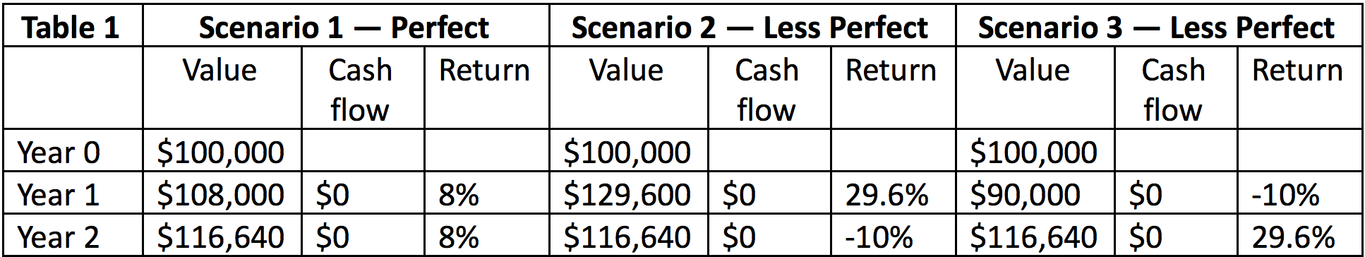
As shown in Table 1, all the three scenarios result in the same investment value of $116,640 at the end of year two. And they all earn the same (geometric) average rate of return of 8 percent.² As long as the average rate of return is 8 percent, return volatility and the order of these returns do not matter. So far, so good.
Example 2: Investing $100,000 in two years with cash outflows in the interim
This example is similar to Example 1, with the same invested amount of money at the beginning and the same annual rates of return for the three scenarios. The only difference is you withdraw $50,000 at the end of year 1.

The three scenarios in this example, as shown in Table 2, have completely different ending investment values. In this case, return volatility and the order of returns significantly affect the investment outcome, even though the average rates of return of the three scenarios are the same (8 percent). Specifically, the scenario where the strong return (29.6 percent) happens in year 1 produces a higher final investment value ($71,640), while the scenario where the weak return (-10 percent) happens first produces a lower final investment value ($51,840). This is because the $50,000 withdrawal at the end of year 1 weakens the effect of the investment return in year 2. As a result, the overall outcome is skewed by the return in the first year.
Example 3: Investing $100,000 in two years with cash inflows in the interim
This example is similar to Example 2. However, instead of withdrawing $50,000, you contribute $50,000 at the end of year 1.
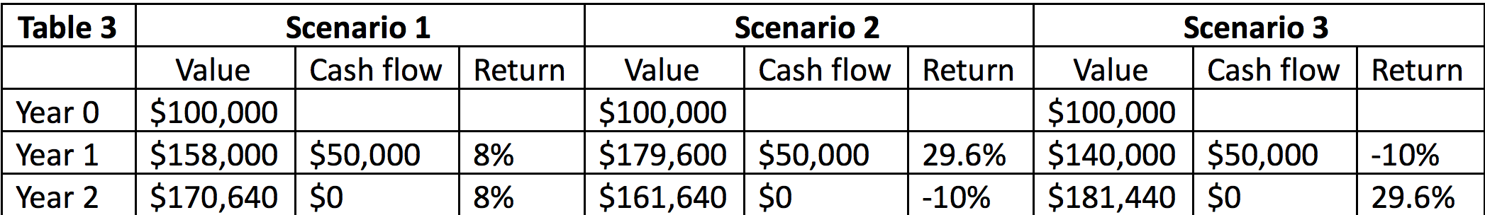
Table 3 shows that, again, return volatility and the order of returns matter. The effects in this example, however, are opposite to those in Example 2. The scenario where the strong return happens first produces a lower final investment value ($161,640), while the scenario where the weak return happens first produces a higher final investment value ($181,440). This is because the $50,000 contribution amplifies the effect of the second year’s investment performance, so the second year’s return is relatively “overweighed” compared to the first year’s.
Funding pension benefits is more like Example 2 and 3, combined, rather than Example 1. A typical pension fund receives contributions (cash inflows) and pays out benefits (cash outflows). These cash flows, combined with volatile investment returns, can produce distorting effects that lead to unexpected funding outcomes even though the fund earns an average rate of return exactly equal to or very close to the return assumption.
One way to capture these cash flow effects in measuring investment performance is to use the money-weighted rate of return (MWRR). The geometric average rate of return we’ve been talking about is actually the time-weighted rate of return (TWRR), which is calculated by isolating investment returns from cash flow effects, then linking these returns geometrically together. The MWRR, on the other hand, is calculated by using a discount rate that equalizes cash inflows and outflows. This discount rate represents the MWRR and is also called the “internal rate of return” (IRR).
Both the TWRR and the MWRR have their strengths and weaknesses:
- The TWRR’s primary advantage is it reflects the true performance of an investment manager because it only counts investment returns in isolation of cash flows. Typically, the investment manager of a pension fund has no control over these cash flows, which are a function of contributions and benefit payments, so it is not fair to use the MWRR in evaluating the manager’s performance.
- On the flip side, the TWRR may not accurately communicate the actual investment returns earned by the pension system as it ignores the cash flows experienced by the system. The MWRR does this job better by incorporating both the size and timing of the cash flows.
Example 4: The City of Austin Employees’ Retirement System
As previously stated, a big problem with most public pension plans is their return assumptions typically ignore the risk that the actual funding outcome will be materially different from the target funding outcome even though the assumed rate of return will be realized in the TWRR form. To illustrate, consider the following example using projections for the City of Austin Employees’ Retirement System (COAERS) for the next 31 years.
First, I assume the plan’s return assumption of 7.5 percent reflects its true geometric long-term expected rate of return. Based on the plan’s target investment portfolio, I estimate that the fund’s annual return volatility measured in standard deviation is about 11 percent. These parameters are then used to generate 10,000 31-year series of random returns, which in turn are put into a COAERS funding model to create 10,000 different funding scenarios. Then I select among these 10,000 scenarios three funding scenarios that have the same 7.5 percent average compound rate of return but different annual return patterns.³ One scenario has strong returns in early years but weak returns in later years. Another scenario has weak returns in early years but strong returns in later years. And another scenario has a mixed timing of strong and weak returns. Figure 1 below shows the trends in the funded ratios of these scenarios.
Figure 1: COAERS’s Projected Funded Ratios Under Four Scenarios
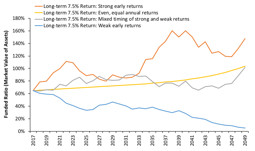
Because COAERS’s statutory funding policy relies on statutorily fixed amounts of contribution as a percentage of payroll rather than on actuarially determined contributions—which can change to accommodate to funding shortfalls/surpluses—the plan’s funded ratio provides a clear signal to compare different scenarios of return patterns.
Figure 1 shows that although all the four scenarios have the same 7.5 percent compound average rate of return or TWRR, they produce very different funding outcomes. The yellow line is what the plan administrators have in mind when they envision the plan’s future in case the 7.5 percent average return is perfectly achieved: a smooth line going from 64 percent to 100 percent. The grey line is what most people envision in case the average rate of return equals 7.5 percent but the annual returns are volatile.
However, most ignore the possibilities of the orange line and the blue line. If the plan earns strong returns in early years but weak returns in later years, the funded ratio will follow a path better than expected (orange line). Conversely, if weak returns happen early followed by strong returns, the funded ratio may get strikingly low (blue line), though the TWRR matches the assumed 7.5 percent.
This is again because of cash flow effects. COAERS is projected to pay more in benefits than they receive in contributions, generating negative cash flows. The negative cash flows, in this case, act like the cash outflow in Example 2, giving more weight to early returns than to later returns. The case is clear when we look at the MWRR. The blue line’s MWRR is only 5.2 percent, compared to the orange line’s MWRR of 8.1 percent. The yellow line and the gray line have about the same MWRR of 7.5 percent.
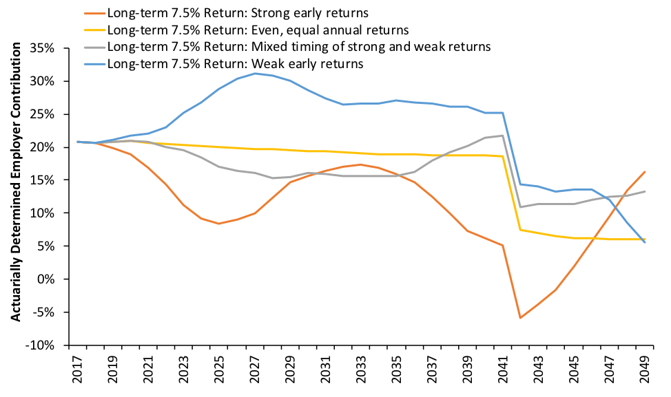
What would happen to these scenarios if the plan switched from the statutory funding policy to an actuarially determined one? The same patterns would emerge from the contribution side, as shown in Figure 2 below. The “strong early returns” scenario enjoys significantly lower employer contribution rates relative to the “weak early returns” scenario. More remarkably, the blue line is entirely above the yellow line, which represents the “perfect” scenario.4
Figure 2: COAERS’s Projected Actuarially Determined Employer Contribution Rates Under Four Scenarios
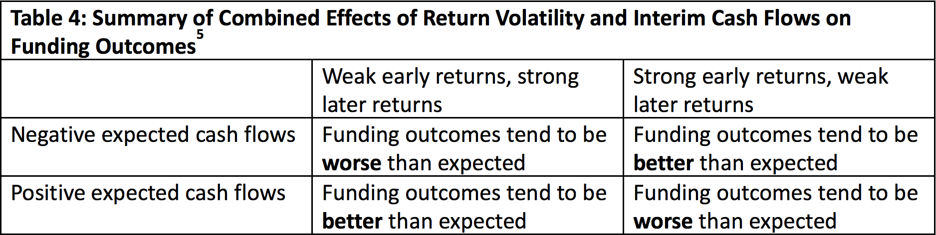
The combined effects of return volatility and interim cash flows on a typical pension plan are summarized in Table 4.
Some may argue that since annual returns are random, the chance of having weak early returns is probably offset by the chance of having strong early returns, so we shouldn’t worry too much about the TWRR vs. MWRR difference. This line of reasoning has two problems. First, the chance of having weak early returns isn’t offset by the chance of having strong early returns any more than the chance of landing heads is offset by the chance of landing tails when tossing a coin. In other words, the probability of bad outcomes doesn’t drop to zero merely because there’s an equal probability of good outcomes.
Second, investment returns for major asset classes over the next 10-15 years are expected to be markedly lower than the historical long-term average. Moreover, the 10-year expected returns are notably lower than the 20-year expected returns, according to a major survey of capital market assumptions. These estimates suggest that the chance of having weak early returns is probably higher than the chance of having strong early returns. For those plans that have negative cash flows, this means the long-term expected MWRR is likely lower than the expected TWRR, and the funding outcomes will be likely worse than expected.
Those concerned about the funding integrity of public pension plans should understand how return volatility and cash flow effects can impact a plan’s financial health. Plan administrators should take into account the TWRR vs. MWRR consideration when thinking about the appropriate return assumption.
- See more discussion about this issue in our paper on the discount rate.
- Because [(1+29.6%)*(1-10%)]^0.5 – 1 = 8%
- Note that not all the 10,000 scenarios have the same 7.5 percent average compound rate of return. These 10,000 scenarios represent a distribution of outcomes, the range of which is positively correlated with the risk of the investment. But the median outcome has an average compound return of about 7.5 percent.
- Some may quibble that the employer contribution rates in this case do not tell the whole story, and one needs to look at the funded ratio too. It’s true that the final funded ratio (in the year 2049) of the “strong early returns” scenario in this case is lower than that of the “weak early returns” scenario. However, the funded ratio of the former scenario is higher than that of the latter one during most of the 31-year period. And most importantly, the “debt financing cost”, measured by the present value of the projected amortization payments plus the present value of the remaining unfunded liability at the end of the year 2049, is lower for the “strong early returns” scenario than for the “weak early returns” scenario.
- “Funding outcomes” here should be taken broadly to mean not just the funded ratio but also the actuarially required contributions, and ultimately the debt financing cost (see footnote 4).
Stay in Touch with Our Pension Experts
Reason Foundation’s Pension Integrity Project has helped policymakers in states like Arizona, Colorado, Michigan, and Montana implement substantive pension reforms. Our monthly newsletter highlights the latest actuarial analysis and policy insights from our team.